
Histogram Done Right: 2KB Memory, 0.2% Error
本文链接: https://blog.openacid.com/algo/histogram/

The Problem: Tracking Request Latency Without Slowing Things Down
When we were building Databend and OpenRaft, we ran into a familiar need: we wanted to see how request latency was distributed across the system, in real time, without burning CPU or memory to do it. This article explains the design behind base2histogram, the library we built to solve it.
Consider the life of a single Raft log entry. It passes through several stages, and each one has its own latency profile:
- Received → written to storage
- Persisted to local disk
- Replicated to remote nodes
- Acknowledged by a majority quorum
- Committed → applied to the state machine
A histogram is the natural tool here — plot latency on the x-axis, request count on the y-axis, and you get an immediate picture of where time is being spent.
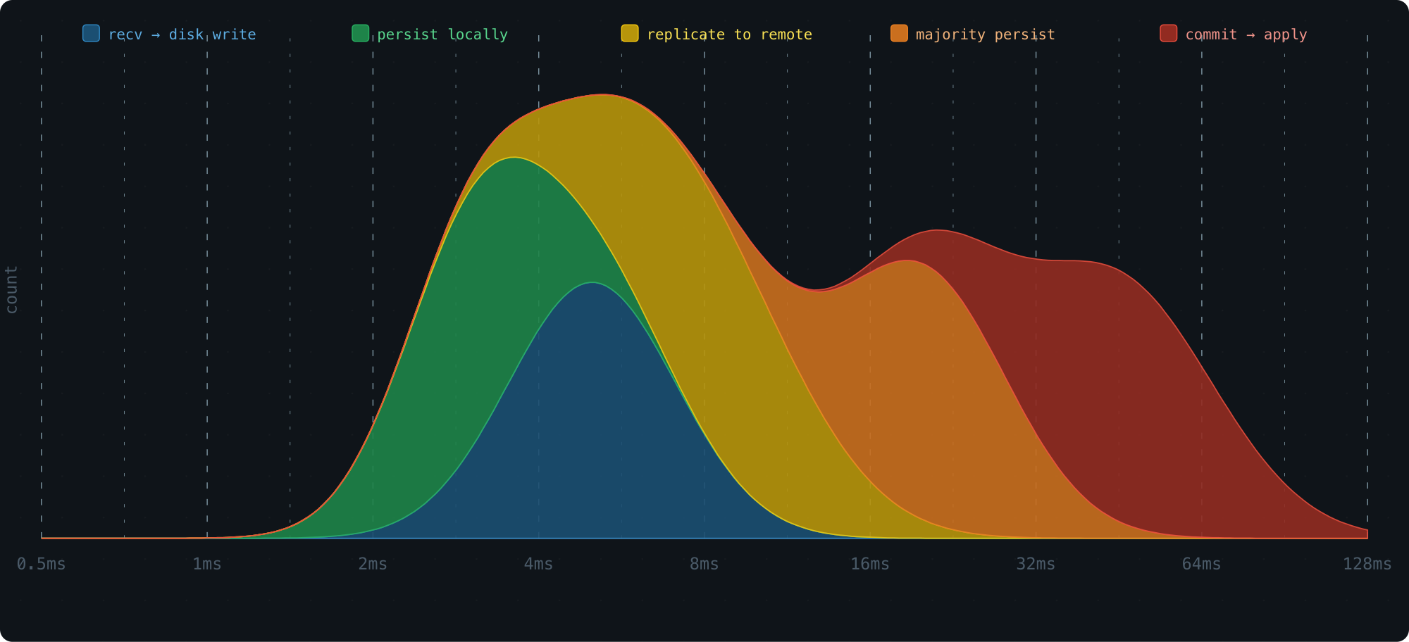
This kind of visibility is what lets you find bottlenecks and fix the right thing.
But there’s a catch: collecting metrics can’t get in the way of doing actual work. So the histogram needs to be:
- O(1) to record — no sorting, no rebalancing, nothing that can stall a hot path
- Tiny in memory — the system may run hundreds or thousands of these at once
- Queryable for percentiles — P50, P95, P99
Let’s walk through how we designed one that hits all three.
Recording: Getting Samples Into Buckets
Why Log-Scale Buckets
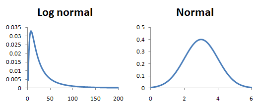
Most requests cluster around some typical latency, with a few outliers on both ends. This is a log-normal distribution — take the log of the latency values, and the shape becomes a classic bell curve.
The signature look: a peak at lower values, then a gradual long tail stretching to the right.
To build a histogram, we divide the x-axis into buckets and count how many samples land in each one.
The key question is how to size those buckets. Equal-width buckets work great for a normal distribution, but latency is log-normal — the data only looks uniform on a logarithmic scale. So the buckets need to grow on a log scale, not a linear one.
The simplest version of this: each bucket is twice as wide as the one before it.
[0,1), [1,2), [2,4), [4,8), [8,16), ...
Why powers of 2? Because multiplying by 2 is free on a CPU, and mapping a value to its bucket takes a single leading zero count instruction.
Simulate a log-normal workload, plot the bucket counts with the bucket index on the x-axis (effectively a log transform), and the result is a clean bell curve:
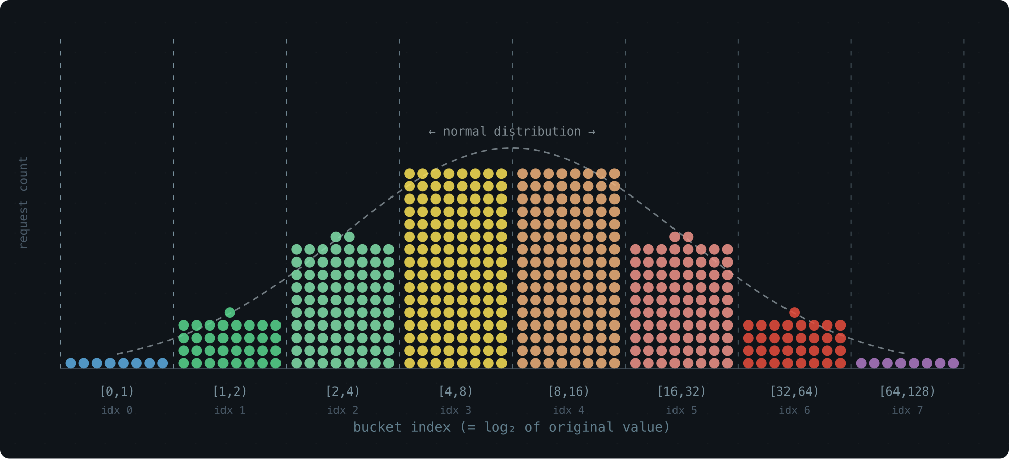
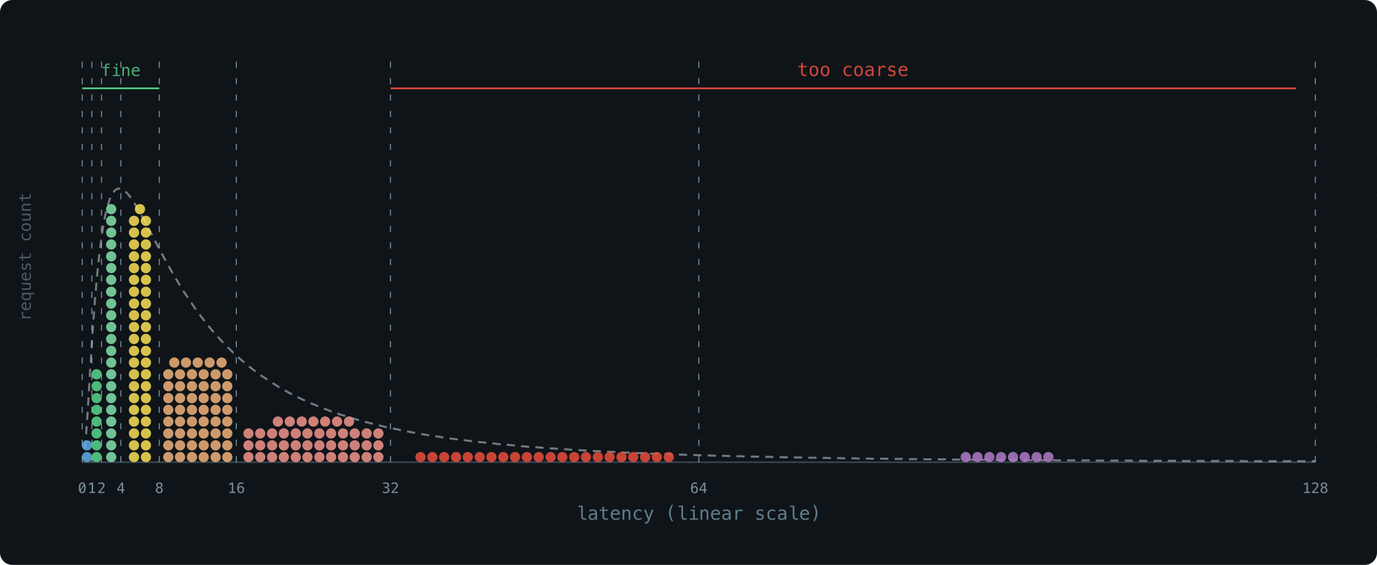
Storage-wise, this is great — 65 buckets cover the entire u64 range. Resolution-wise, not so much. The last bucket spans half of all possible values. Everything that lands there is a blur.
A Tempting Fix We Passed On
An obvious improvement: use a smaller growth factor, like 1.1× instead of 2×. More buckets, finer resolution:
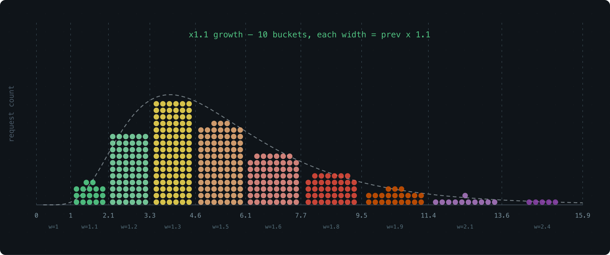
The problem is cost. Finding the right bucket for a value l means solving for the smallest x where 1 + 1.1 + 1.1^2 + ... + 1.1^x >= l — and that requires floating-point logarithms. That’s real overhead on a hot path.
We wanted to stay in the world of integers and bit operations.
The Trick: Float-Like Encoding
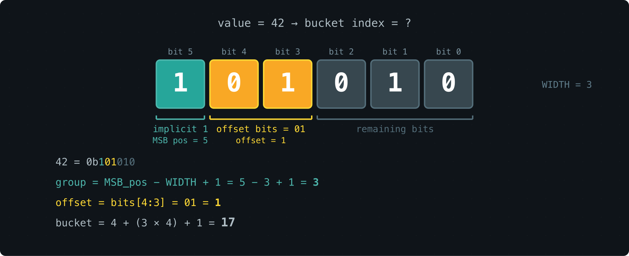
Here’s the idea that makes everything work. We keep the roughly exponential bucket sizes, but we encode each bucket using a fixed number of bits — a parameter we call WIDTH.
Think of a bucket’s lower bound as a tiny floating-point number. The MSB position gives you the exponent (which group of buckets you’re in), and the next few bits give you the offset within that group.
With WIDTH=3 (the default), a bucket boundary looks like this in binary:
00..00 1 xx 00..00
       |
       MSB
<- significant
The position of the leading 1 picks the group. The two bits that follow pick the bucket within the group.
Here’s what the first few groups look like — each bucket is fully described by just 3 bits:
WIDTH = 3:
range bucket index bucket size
[0, 1) 0 0b0 ..... 000 1
[1, 2) 1 0b0 ..... 001 1
[2, 3) 2 0b0 ..... 010 1
[3, 4) 3 0b0 ..... 011 1
[4, 5) 4 0b0 ..... 100 1
[5, 6) 5 0b0 ..... 101 1
[6, 7) 6 0b0 ..... 110 1
[7, 8) 7 0b0 ..... 111 1
[8, 10) 8 0b0 .... 1000 2
[10, 12) 9 0b0 .... 1010 2
[12, 14) 10 0b0 .... 1100 2
[14, 16) 11 0b0 .... 1110 2
[16, 20) 12 0b0 ... 10000 4
[20, 24) 13 0b0 ... 10100 4
[24, 28) 14 0b0 ... 11000 4
[28, 32) 15 0b0 ... 11100 4
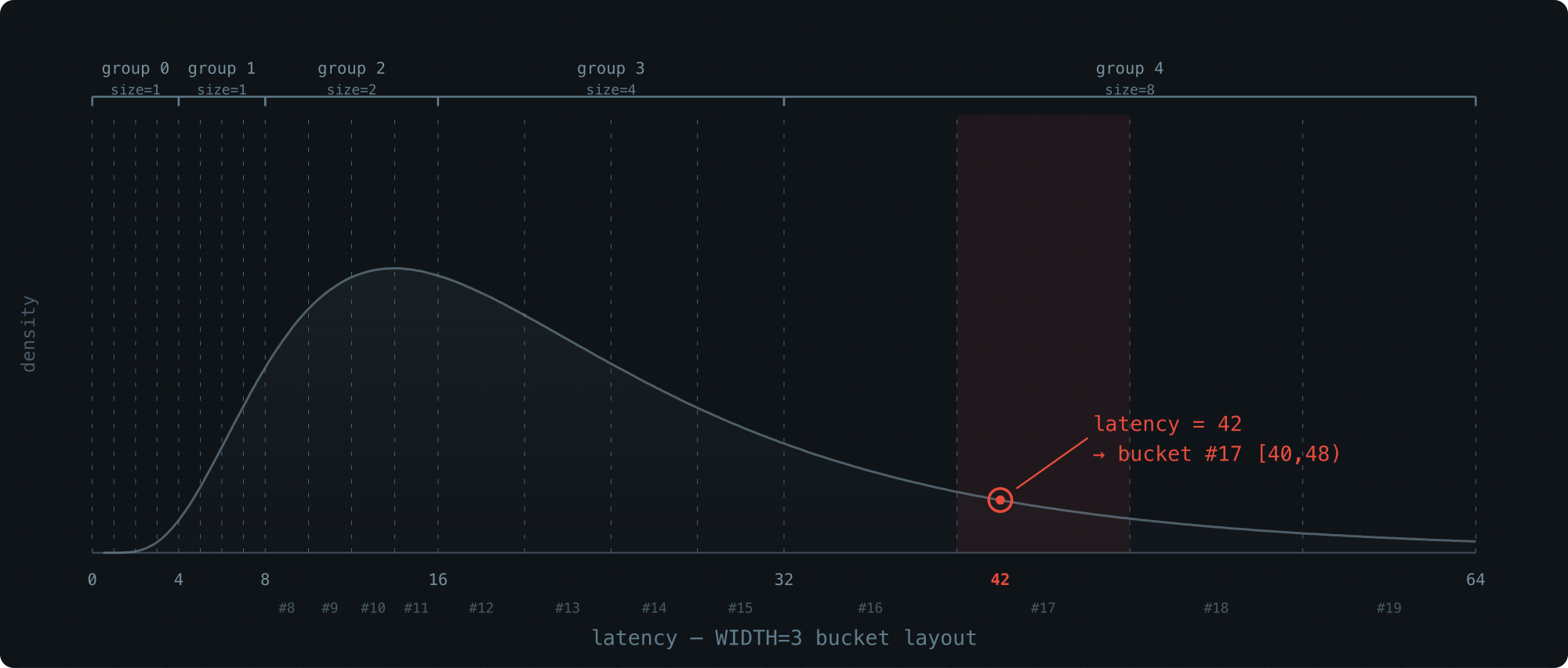
[32, 40) 16 0b0 .. 100000 8
[40, 48) 17 0b0 .. 101000 8
[48, 56) 18 0b0 .. 110000 8
[56, 64) 19 0b0 .. 111000 8
The pattern is clean:
- Each group contains
2^(WIDTH-1) = 4buckets - The 2 bits after the MSB select the bucket within the group
- It’s a 3-bit float: 1 implicit leading bit + 2 fractional bits
Bucket sizes grow roughly logarithmically, and computing the bucket index is just a matter of extracting the top WIDTH bits — a handful of integer and bit ops. Recording a sample is O(1).
Walk-through with latency = 42:
value = 42 (binary: 0b101010)
  MSB position: 5
  group: 5 - 2 = 3
  2 bits after MSB: 01 (from 1[01]010)
  offset in group: 1
  Bucket index: 4 + (3 × 4) + 1 = 17
Tuning WIDTH: The Precision–Memory Knob
WIDTH sets how many buckets each group gets (2^(WIDTH-1)).
Groups top out at 64 (they still double in size, covering the full u64 range).
Here’s how the trade-off plays out:
| WIDTH | Buckets | Mem/slot | Buckets per group |
|---|---|---|---|
| 1 | 65 | 520 B | 1 |
| 2 | 128 | 1.0 KB | 2 |
| 3 | 252 | 2.0 KB | 4 (default) |
| 4 | 496 | 3.9 KB | 8 |
| 5 | 976 | 7.6 KB | 16 |
| 6 | 1920 | 15.0 KB | 32 |
At the default WIDTH=3, one histogram costs 2 KB and records every sample in O(1).
That’s the write side sorted. Now for the read side.
Percentile Estimation: Getting Answers Out
Once we’ve collected the counts, we want percentiles: at what latency have 50% of requests finished (P50)? 90% (P90)? 99% (P99)?
Locating the Right Bucket
The basic idea is simple.
For P50: count the total samples, take 50% to get a target rank p, then walk through the buckets from the start, accumulating counts until you pass p. That’s your bucket.
But a bucket spans a range, not a point. We still need to estimate where inside the bucket the percentile actually falls.
Here are a few ways to do that, from rough to precise. All error numbers below come from a log-normal distribution (API latency scenario), WIDTH=3, 1,000,000 samples.
Midpoint: just return (min + max) / 2.
Many histogram libraries do this (e.g., iopsystems/histogram).
It’s a blind guess — it ignores everything about how samples are distributed within the bucket.
| P50 | P95 | P99 | |
|---|---|---|---|
| midpoint | 5.018% | 7.732% | 4.861% |
Uniform interpolation: assume samples are spread evenly across the bucket (a flat rectangle), then interpolate linearly: estimate = min + (max - min) × rank / count.
Better than midpoint — at least it uses where in the bucket the target rank falls. But “evenly spread” is a rough assumption. Log-normal data is skewed even within a single bucket.
Trapezoid Interpolation (Our Approach)
Uniform interpolation treats the density inside a bucket as flat. In reality, it’s sloped — denser on the side closer to the peak of the distribution.
If we know which way the density tilts, we can swap the rectangle for a trapezoid and land much closer to the true value.
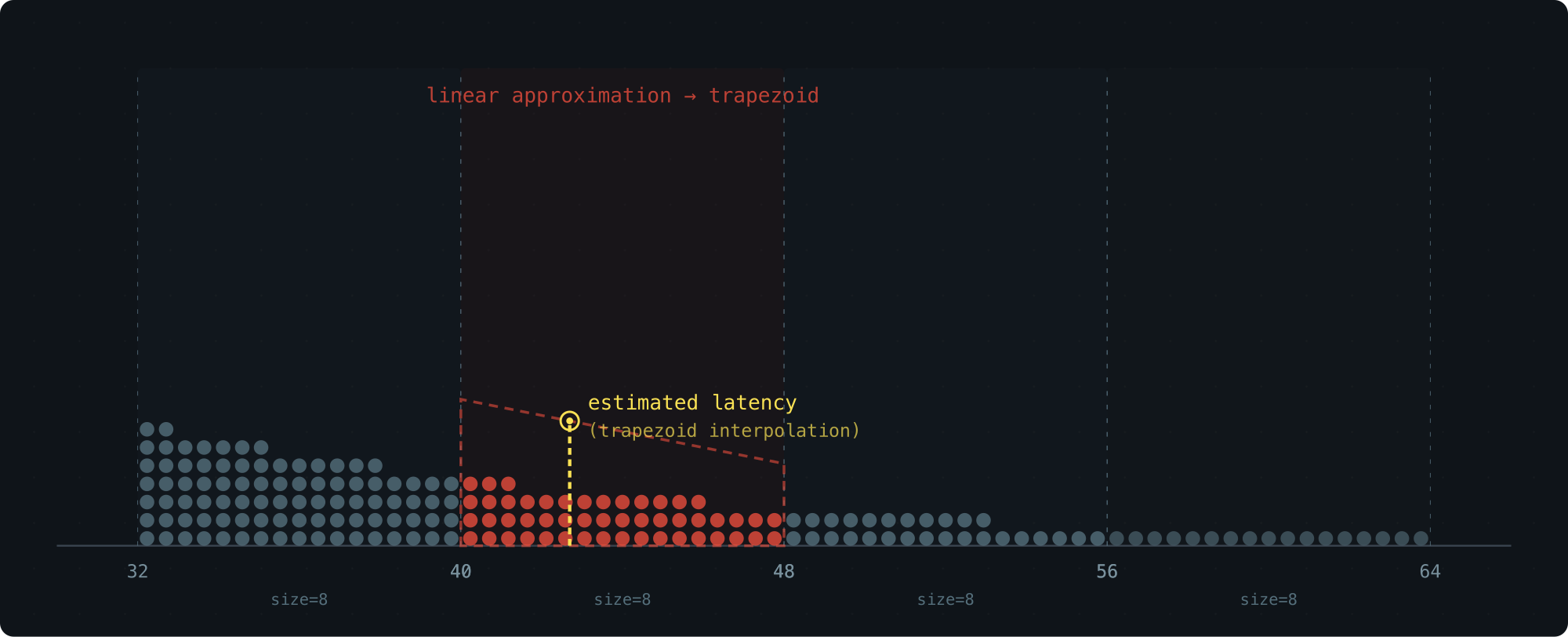
Each bucket stores only a count — we don’t want to add extra fields. So where does the slope information come from? The neighbors.
The densities of the left and right buckets tell us how the density slopes through the current bucket.
Here’s the recipe.
Compute the average density of the left bucket: d0 = c0/(x1-x0), and treat it as the density at that bucket’s midpoint m0.
Do the same for the right bucket: d2 = c2/(x3-x2) at midpoint m2.
Assume density varies linearly from m0 to m2 — over this short range, that’s a reasonable approximation.
This gives us the slope k.
Inside the target bucket, the density now forms a trapezoid: a sloped line with slope k, pinned so that the density at the bucket’s midpoint (x1+x2)/2 equals the bucket’s own average density d1 = c1/(x2-x1) (the midpoint of a linear function always equals its average).
To find the percentile, we solve for the x-position where the trapezoid’s area from x1 equals the target rank.
Same distribution, same buckets — here’s how it stacks up:
| P50 | P95 | P99 | |
|---|---|---|---|
| midpoint | 5.018% | 7.732% | 4.861% |
| trapezoid | 0.000% | 0.080% | 0.086% |
Two orders of magnitude better, with zero additional storage.
The three-bucket layout:
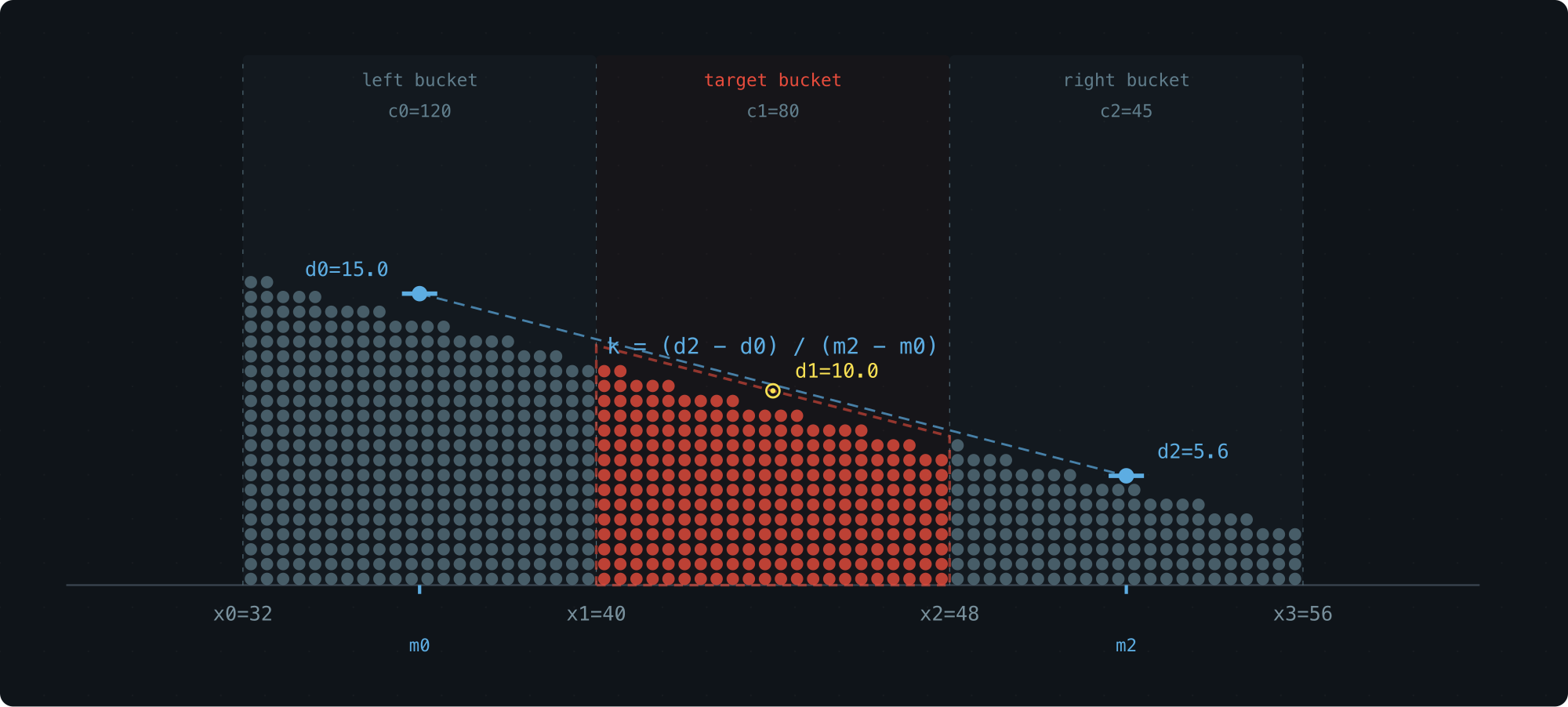
| Variable | Meaning |
|---|---|
x0, x1, x2, x3 |
Boundaries of the three adjacent buckets |
w0, w1, w2 |
Bucket widths: w0 = x1-x0, w1 = x2-x1, w2 = x3-x2 |
c0, c1, c2 |
Sample counts in each bucket |
rank |
How many samples into the target bucket the percentile falls |
d0 = c0 / w0       -- left bucket density
d1 = c1 / w1       -- target bucket density
d2 = c2 / w2       -- right bucket density
Midpoints of the left and right buckets: m0 = (x0+x1)/2, m2 = (x2+x3)/2.
Slope:
k = (d2 - d0) / (m2 - m0)
Then solve for the x-position where the trapezoid’s cumulative area from x1 equals the rank.
The whole thing runs on three counts and their bucket boundaries. Nothing else stored, nothing else needed.
Benchmarks: Seven Distributions, Six WIDTH Settings
We tested across 7 representative distributions with 1,000,000 samples each, using trapezoid interpolation.
The rows to watch are LN-API and LN-DB at W=3 — these are the real-world latency cases, running on the default 2 KB configuration:
|                   W=1      W=2      W=3      W=4      W=5      W=6
| ------------------------------------------------------------------
| Uniform P50    0.108%   0.028%   0.012%   0.018%   0.019%   0.002%
|         P95    2.317%   1.988%   1.035%   0.475%   0.005%   0.005%
|         P99    4.290%   4.129%   3.706%   1.486%   0.298%   0.162%
|
| LN-API  P50    2.281%   0.182%   0.000%   0.000%   0.000%   0.000%
|         P95   20.256%   3.963%   0.080%   0.040%   0.040%   0.000%
|         P99   11.951%   3.594%   0.086%   0.000%   0.029%   0.000%
|
| Bimodal P50    1.381%   0.394%   0.394%   0.197%   0.197%   0.197%
|         P95    3.918%   0.172%   0.012%   0.028%   0.038%   0.008%
|         P99    1.521%   1.344%   0.543%   0.078%   0.016%   0.014%
|
| Expon   P50    1.012%   0.000%   0.145%   0.145%   0.145%   0.000%
|         P95   10.989%   0.200%   0.000%   0.000%   0.033%   0.033%
|         P99   18.665%   4.574%   0.824%   0.022%   0.022%   0.022%
|
| LN-DB   P50    2.018%   0.034%   0.000%   0.000%   0.000%   0.034%
|         P95    2.027%   0.368%   0.039%   0.006%   0.019%   0.026%
|         P99    3.764%   1.066%   0.187%   0.007%   0.003%   0.062%
|
| Sequent P50    0.095%   0.000%   0.000%   0.000%   0.000%   0.000%
|         P95    2.271%   1.967%   1.011%   0.496%   0.000%   0.000%
|         P99    4.272%   4.118%   3.696%   1.521%   0.305%   0.169%
|
| Pareto  P50   10.127%   1.899%   0.633%   0.633%   0.633%   0.000%
|         P95    9.239%   0.272%   0.000%   0.136%   0.000%   0.000%
|         P99    3.517%   0.879%   0.231%   0.093%   0.046%   0.046%
|
| ------------------------------------------------------------------
| Buckets            65      128      252      496      976     1920
| Mem/slot        520 B   1.0 KB   2.0 KB   3.9 KB   7.6 KB  15.0 KB
| Mem total      1.0 KB   2.0 KB   3.9 KB   7.8 KB  15.2 KB  30.0 KB
What each distribution models:
- Uniform (uniform distribution): synthetic benchmarks
- LN-API (log-normal σ=0.5): API and microservice latency
- Bimodal (bimodal distribution): cache hit/miss — 90% fast path ~500μs, 10% slow path ~50ms
- Expon (exponential distribution): network and I/O waits
- LN-DB (log-normal σ=1.0): database query latency, with a wider tail
- Sequent (sequential): adversarial worst case
- Pareto (Pareto distribution α=1.5): heavy-tailed workloads like request sizes
For the latency distributions we care about most — LN-API and LN-DB — WIDTH=3 delivers sub-0.2% error on 2 KB of memory.
Summary
- 2 KB memory (WIDTH=3, 252 buckets of u64), P50/P95/P99 error under 0.2% for log-normal latency
- O(1) recording, O(buckets) querying
- Trapezoid interpolation is what makes it work — over 10× more accurate than midpoint, with zero extra storage
- WIDTH is tunable: 520 B for bare-minimum tracking, up to 15 KB for maximum precision
- Code: base2histogram
Reference:
-
Databend : https://github.com/databendlabs/databend
-
MSB : https://en.wikipedia.org/wiki/Bit_numbering#Most_significant_bit
-
OpenRaft : https://github.com/databendlabs/openraft
-
Pareto distribution : https://en.wikipedia.org/wiki/Pareto_distribution
-
base2histogram : https://github.com/drmingdrmer/base2histogram
-
bimodal distribution : https://en.wikipedia.org/wiki/Multimodal_distribution
-
exponential distribution : https://en.wikipedia.org/wiki/Exponential_distribution
-
floating-point number : https://en.wikipedia.org/wiki/Floating-point_arithmetic
-
histogram : https://en.wikipedia.org/wiki/Histogram
-
iopsystems/histogram : https://github.com/iopsystems/histogram
-
leading zero counting : https://en.wikipedia.org/wiki/Find_first_set#CLZ
-
log scale : https://en.wikipedia.org/wiki/Logarithmic_scale
-
log-normal distribution : https://en.wikipedia.org/wiki/Log-normal_distribution
-
long tail : https://en.wikipedia.org/wiki/Long_tail
-
normal distribution : https://en.wikipedia.org/wiki/Normal_distribution
-
percentile : https://en.wikipedia.org/wiki/Percentile
-
uniform distribution : https://en.wikipedia.org/wiki/Continuous_uniform_distribution
本文链接: https://blog.openacid.com/algo/histogram/

留下评论